Port Traffic Intelligence Platform
A major port authority had no automated way to count or classify vehicles entering its facilities, relying on manual tallying at two high-traffic entrances.
Computer Vision • ML Pipeline Design • Edge Computing • IoT Integration • Data Engineering • Systems Integration


Background
The port authority needed real-time vehicle counts and classification across two entrances to support traffic planning, dwell time analysis, and future routing decisions. Manual tallying was inconsistent, labor-intensive, and produced no structured data.
No off-the-shelf traffic counting system could classify the range of vehicles that operate in a port environment. Standard passenger vehicle models miss the heavy equipment, specialized trucks, and mixed-class traffic patterns unique to port operations.
The Solution
I designed, developed, and deployed the full detection and tracking pipeline for the port authority. After the initial delivery, I integrated the system into the company’s platform and deployed it at both entrances.
The system runs a custom-trained object detection model on edge hardware at each entrance, classifying vehicles across 12 port-specific classes in real time. Detection events feed into dashboards and downstream services.
Deep Dive: ML Pipeline & Edge Deployment
Architecture
The system operates as an edge-first pipeline with no cloud dependency for inference. Each entrance runs a camera connected to a Jetson Nano running the detection model. A Raspberry Pi handles network routing and LTE connectivity to the central server. Detection events publish over MQTT into the company's IoT platform, which distributes data to dashboards, reporting, and a license plate correlation service.
After the capstone, I integrated detection output into the company's existing web platform and built an ML metrics dashboard to show model performance and detection trends.
Data Engineering
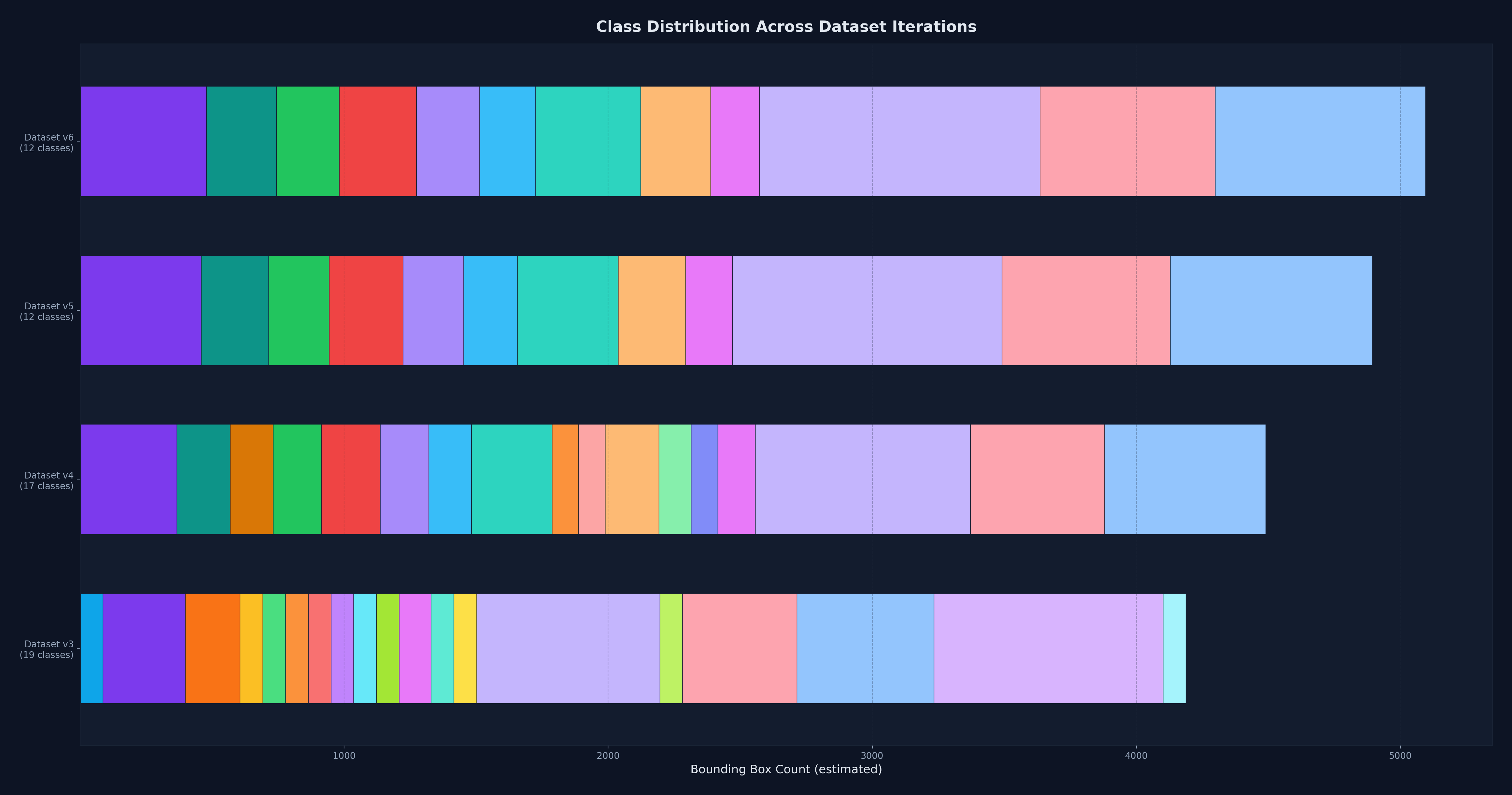
The dataset went through six full iterations before the model performed reliably in production conditions. Each iteration addressed failures discovered during field testing, not just accuracy metrics on held-out data.
I collected training data from camera feeds at the port entrances by downloading motion-triggered video clips, each roughly 20 seconds long. I stitched clips in groups of 100 for annotation in CVAT (Computer Vision Annotation Tool), then labeled all training data manually.
The initial class list started at 19 vehicle types based on port operations requirements. Through iterative testing, I found that many classes were visually indistinguishable at the camera's resolution and angle. Cement trucks and freight trucks viewed head-on are one solid color with no distinctive features. Dump trucks with different cargo look identical from above. The real challenge was getting the categorization right, not just reducing the count. Classes had to be both learnable by the model and meaningful to port operations. I met with the port authority to understand which distinctions mattered operationally, then restructured the class list over four dataset revisions. The final set settled at 12 classes.
By the sixth iteration, the training set contained approximately 5,000 labeled samples. Class imbalance was a recurring problem. Some vehicle types appeared rarely but were operationally important. I balanced the data through targeted collection during busy shifts, image augmentation, and negative samples to suppress false positives from cement and freight trucks.
The camera's position meant large vehicles were only partially visible for much of their time in the frame, depending on the vehicle type and size. A truck entering from the top shows only a cab, then gradually reveals its body as it moves through. I initially tried stitching partial frames to reconstruct full vehicles, but perspective distortion made the composites unreliable and lowered accuracy. Instead, I labeled vehicles at the point where they were most visible in the frame and trained the model to classify from those partial views.
Model Selection and Training
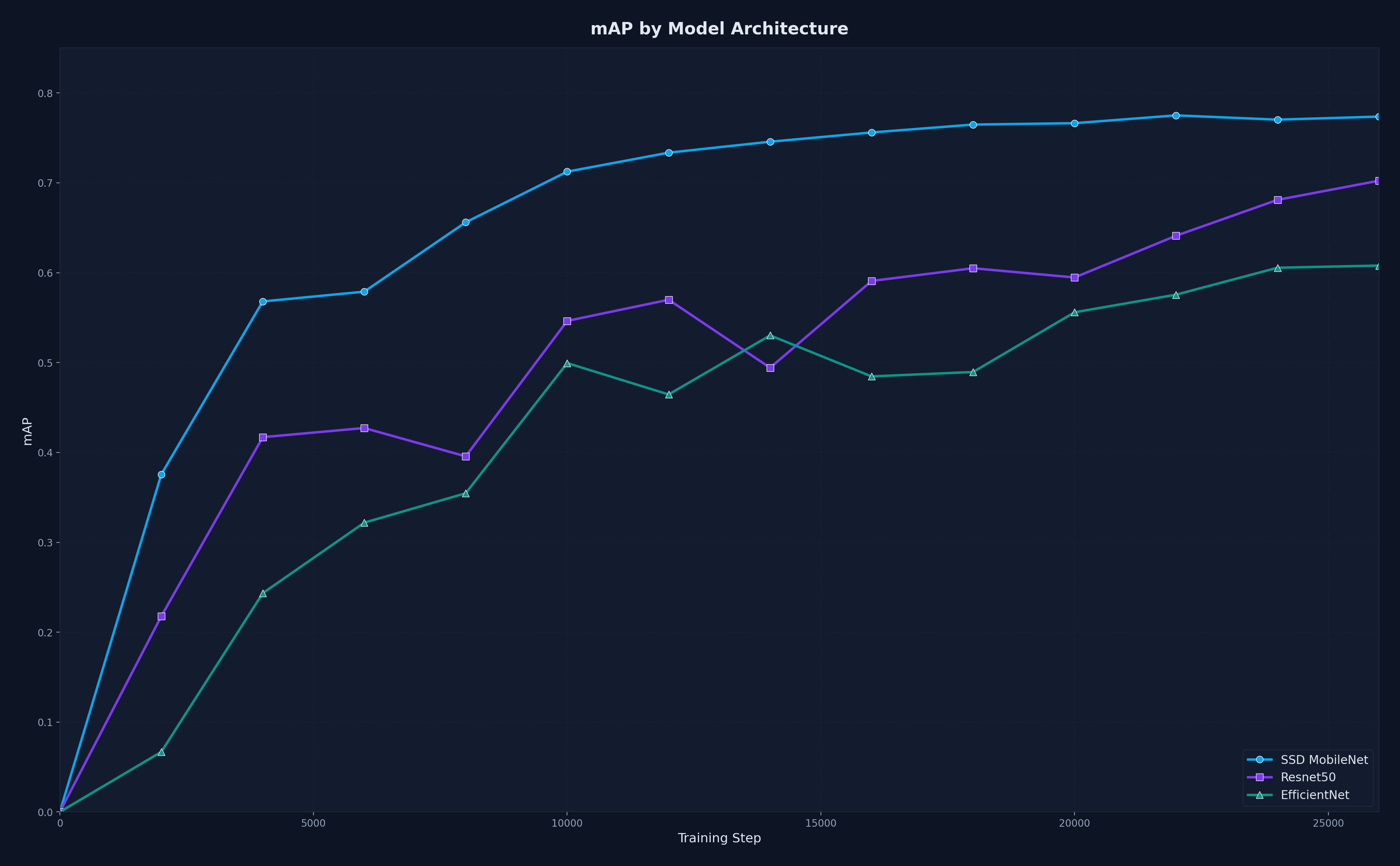
I evaluated six detection architectures against the constraints of the Jetson Nano. SSD MobileNet V2 FPNLite 640x640 outperformed the others in a comparison experiment. MobileNet's lightweight design kept inference fast, and its feature pyramid layer handled the range of vehicle sizes in the scene.
Training used the TensorFlow Object Detection API. I tracked loss convergence, per-class AP, and confusion matrices across all six dataset iterations. Each iteration's model was field-tested before the next round of data collection began. The classification loss consistently exceeded the localization loss. The model had no trouble finding vehicles. The difficulty was telling them apart.
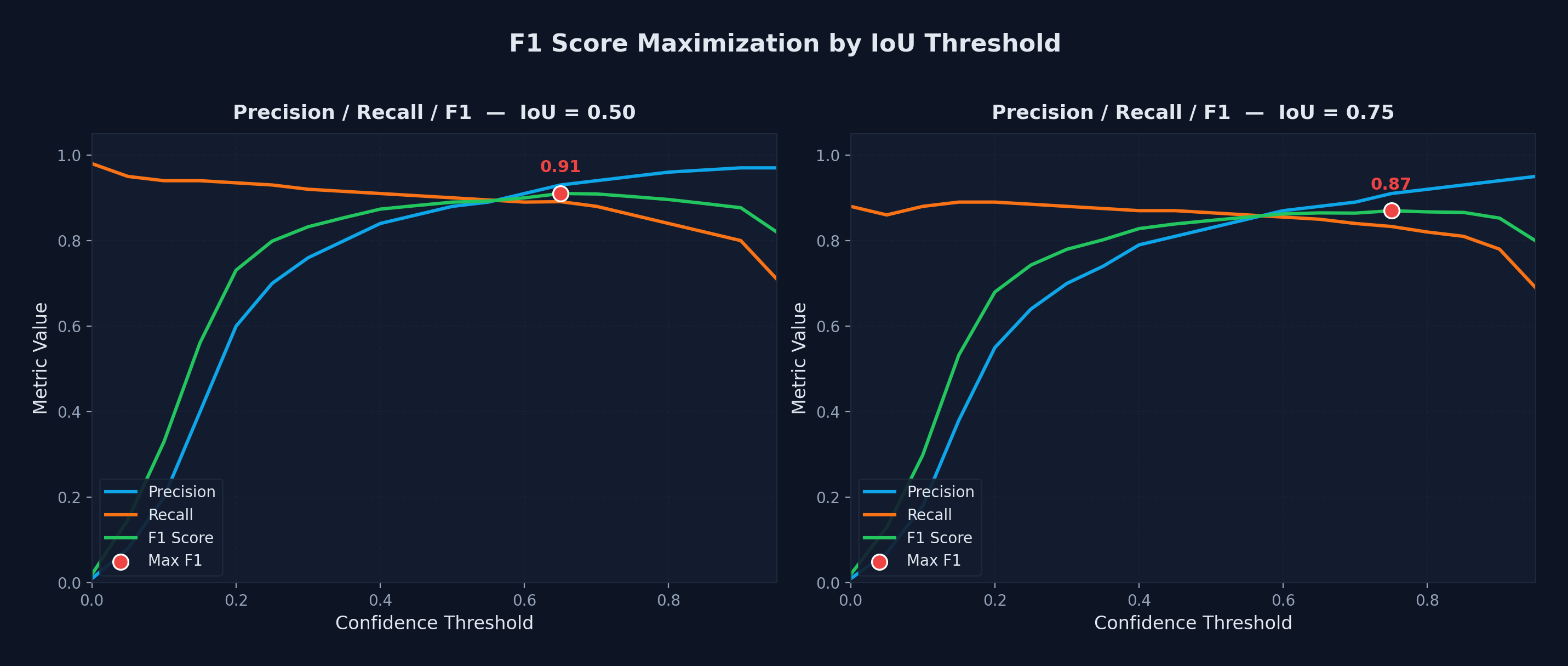
I set the IoU threshold by sweeping confidence values and picking the point where the F1 score peaked. At IoU 0.50, the best F1 was 0.92 and at IoU 0.75 it was 0.88. This gave a clean balance between precision and recall without manual tuning.
For deployment on the Jetson Nano, I used the 320x320 variant of the same architecture. The smaller input maintained the same 91% precision, recall, and F1 across all 12 classes while fitting within the Nano's compute budget.
Tracking and Counting
Detection alone does not produce a count. The same vehicle appears in multiple consecutive frames and must be tracked as one object across the camera's field of view.
I implemented a modified SORT tracker with a Kalman filter for position prediction. The tracker matches detections to tracked objects frame by frame and determines the final class label from the distribution of predictions across a track's lifetime. A virtual counting line marks when a tracked object has fully entered or exited the port. Counting events, not raw detections, are what get sent downstream as JSON over MQTT.
Inference Optimization
The trained 320x320 model ran at 2 fps on the Jetson Nano including pre-processing and post-processing. That was unusable for real-time counting.
Pipelining bought the first gain. I split pre-processing, inference, and post-processing into three separate threads so each stage could run concurrently on the next frame. This brought throughput to 7 fps.
TensorRT brought the rest. I converted the TensorFlow saved model to ONNX, then built a TensorRT engine at FP16 precision. The combination of pipelining and TensorRT optimization brought inference to 26 fps, well above the 15 fps minimum requirement.
The conversion pipeline (TF saved model to ONNX to TensorRT) required ONNX-GraphSurgeon for graph manipulation and PyCUDA for memory management. FP16 on the 320x320 model did exaggerate false positives for cement and freight trucks, which I eliminated by adding negative samples to the training data. I pioneered the model optimization pipeline, which became a template for future edge deployments across the company
Edge Deployment
The hardest part of edge deployment was the Nano's dependency environment. The JetPack image runs old, version-locked releases of CUDA, cuDNN, and TensorRT that do not match standard Python packages. Most GPU libraries need to be built from source for the Nano's ARM architecture. I wrote Python scripts that automated the full dependency chain from a clean image: installing GPU libraries at the correct versions, building PyCUDA from source, and sequencing every install precisely to avoid silent version conflicts.
The devices could not be removed from the site, so I built an update script that applied changes in place without reimaging. I worked with the company's hardware and software team to integrate these scripts into their device imaging pipeline, making the setup reusable across other projects.